This is the AR & FOXA1 notebook executed end to end with genomeblocks 2.0, with its figures and result tables. The previous pages explain the concepts; this one shows the actual run. Source:
examples/ar_foxa1_lncap/.
AR & FOXA1 in LNCaP (±DHT)
How the androgen receptor (AR) cistrome depends on the pioneer factor FOXA1 after androgen (DHT) stimulation in LNCaP cells.
Data are ChIP-Atlas (hg38) peaks + bigwigs — run ./download_data.sh first.
LNCaP, 0h vs 4h DHT, for FOXA1, AR, and ATAC-seq (two ATAC replicates / condition).
Note — FOXA1 4h peaks use
SRX23002841.05.bed(matching the FOXA1 4h bigwig). The reference paths in the next cell point at the lackgrp cluster; edit them for your environment.
0. Setup — paths & helpers
import os, time
from contextlib import contextmanager

import numpy as np
import matplotlib.pyplot as plt
from tqdm import tqdm

import genomeblocks as gb
from genomeblocks import Loci, Genes, Atlas, tmm, browser
from genomeblocks.signal_draw import plot_heatmap
from genomeblocks.motifs import scan_motifs_matrix, bootstrap_enrichment


@contextmanager
def timer(label):
    """Print a step's wall-clock time."""
    t0 = time.perf_counter()
    print(f"\u25b6 {label} ...")
    try:
        yield
    finally:
        print(f"\u2713 {label} \u2014 {time.perf_counter() - t0:.1f}s")


# --- downloaded data (see download_data.sh) ---
DATA = "data"
DATA
SRX = {
    "FOXA1_0h": "SRX23002839", "FOXA1_4h": "SRX23002841",
    "AR_0h":    "SRX23002834", "AR_4h":    "SRX23002836",
    "ATAC_0h_r1": "SRX23002894", "ATAC_0h_r2": "SRX23002895",
    "ATAC_4h_r1": "SRX23002898", "ATAC_4h_r2": "SRX23002899",
}
PEAK = {k: f"{DATA}/{s}.05.bed" for k, s in SRX.items()}
BW   = {k: f"{DATA}/{s}.bw"     for k, s in SRX.items()}

# --- hg38 references (edit for your environment) ---
GENOME_FA   = "/groups/lackgrp/genome_annotations/hg38/hg38.fa"
GTF         = "/groups/lackgrp/genome_annotations/hg38/gencode.v49.annotation_protein_coding.gtf"
MOTIF_DB    = "/groups/lackgrp/databases/motifs/motif-db/H14CORE_jaspar_format_lightmotif.txt"
CHROMSIZES  = "/groups/lackgrp/genome_annotations/hg38/hg38_chr.chrom.sizes"
GIGGLE_META = "/groups/lackgrp/databases/giggle/giggle_hg38/hg38_tfs_meta.tsv"
GIGGLE_DIR  = "/groups/lackgrp/databases/giggle/giggle_hg38/ChIP-Atlas-ALL"
1. Load peaks
with timer("load peak files"):
    peaks = {k: Loci.make(v) for k, v in PEAK.items()}

for k, v in peaks.items():
    print(f"{k:12} {len(v):>8,} peaks")
▶ load peak files ...
✓ load peak files — 3.5s
FOXA1_0h        8,657 peaks
FOXA1_4h       10,870 peaks
AR_0h             910 peaks
AR_4h           3,645 peaks
ATAC_0h_r1     53,671 peaks
ATAC_0h_r2     62,741 peaks
ATAC_4h_r1     47,780 peaks
ATAC_4h_r2     51,196 peaks
2. Accessible chromatin — union of ATAC peaks
Concatenate the four ATAC peak sets (both conditions, both reps) and merge()
overlapping intervals into one accessible-region set (the result comes back in
genome order).
with timer("ATAC union (accessible regions)"):
    accessible = (peaks["ATAC_0h_r1"] + peaks["ATAC_0h_r2"]
                  + peaks["ATAC_4h_r1"] + peaks["ATAC_4h_r2"]).merge()

print(f"accessible regions (merged): {len(accessible):,}")
▶ ATAC union (accessible regions) ...
✓ ATAC union (accessible regions) — 0.1s
accessible regions (merged): 72,470
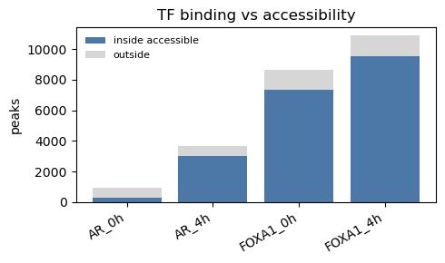
3. AR / FOXA1 binding inside vs outside accessible chromatin
rows = []
for name in ["AR_0h", "AR_4h", "FOXA1_0h", "FOXA1_4h"]:
    s = peaks[name]
    inside = len(s & accessible)              # peaks overlapping accessible
    total = len(s)
    rows.append((name, inside, total - inside))
    print(f"{name:10} {100 * inside / total:5.1f}% inside accessible ({inside:,}/{total:,})")

names = [r[0] for r in rows]
ins   = np.array([r[1] for r in rows])
outs  = np.array([r[2] for r in rows])
fig, ax = plt.subplots(figsize=(5, 3))
ax.bar(names, ins,  label="inside accessible", color="#4c78a8")
ax.bar(names, outs, bottom=ins, label="outside", color="#d6d6d6")
ax.set_ylabel("peaks"); ax.legend(frameon=False, fontsize=8)
ax.set_title("TF binding vs accessibility")
plt.xticks(rotation=30, ha="right"); plt.tight_layout()
AR_0h       31.2% inside accessible (284/910)
AR_4h       83.0% inside accessible (3,027/3,645)
FOXA1_0h    85.0% inside accessible (7,362/8,657)
FOXA1_4h    88.0% inside accessible (9,561/10,870)
4. Keep only accessible TF peaks
with timer("filter TF peaks to accessible"):
    F0 = peaks["FOXA1_0h"] & accessible
    F4 = peaks["FOXA1_4h"] & accessible
    A4 = peaks["AR_4h"]    & accessible

print(f"accessible  FOXA1 0h={len(F0):,}  FOXA1 4h={len(F4):,}  AR 4h={len(A4):,}")
▶ filter TF peaks to accessible ...
✓ filter TF peaks to accessible — 0.0s
accessible  FOXA1 0h=7,362  FOXA1 4h=9,561  AR 4h=3,027
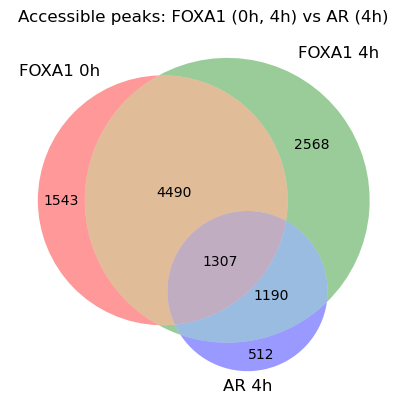
5. Venn — FOXA1 (0h, 4h) vs AR (4h)
To venn genomic intervals we merge all peaks into a shared region universe,
then label each region by which input set overlaps it (overlap_any gives one
boolean per universe row; the row numbers are the region ids). From this:
- AR+F = AR 4h peaks that overlap FOXA1 (0h or 4h) — FOXA1-dependent AR
- AR−F = AR 4h peaks that overlap no FOXA1 peak — FOXA1-independent AR
from matplotlib_venn import venn3

def venn_id_sets(sets):
    """Merge all peaks into a region universe; return one set of region-ids per
    input set (the ids it overlaps) so matplotlib_venn can count the regions."""
    universe = sum(sets[1:], sets[0]).merge()
    return [set(np.flatnonzero(universe.overlap_any(s)).tolist()) for s in sets]

with timer("venn3 membership"):
    ids = venn_id_sets([F0, F4, A4])

fig, ax = plt.subplots(figsize=(5, 5))
venn3(ids, set_labels=["FOXA1 0h", "FOXA1 4h", "AR 4h"], ax=ax)
ax.set_title("Accessible peaks: FOXA1 (0h, 4h) vs AR (4h)")
plt.show()
▶ venn3 membership ...
✓ venn3 membership — 0.0s
with timer("define AR+F / AR-F"):
    F_any = (F0 + F4).merge()            # FOXA1-bound at either timepoint
    ARpF  = A4 & F_any                   # AR 4h that IS FOXA1-bound
    ARmF  = A4 - F_any                   # AR 4h that is NOT FOXA1-bound

print(f"AR+F (FOXA1-dependent): {len(ARpF):,}   AR-F (FOXA1-independent): {len(ARmF):,}")
▶ define AR+F / AR-F ...
✓ define AR+F / AR-F — 0.0s
AR+F (FOXA1-dependent): 2,515   AR-F (FOXA1-independent): 512
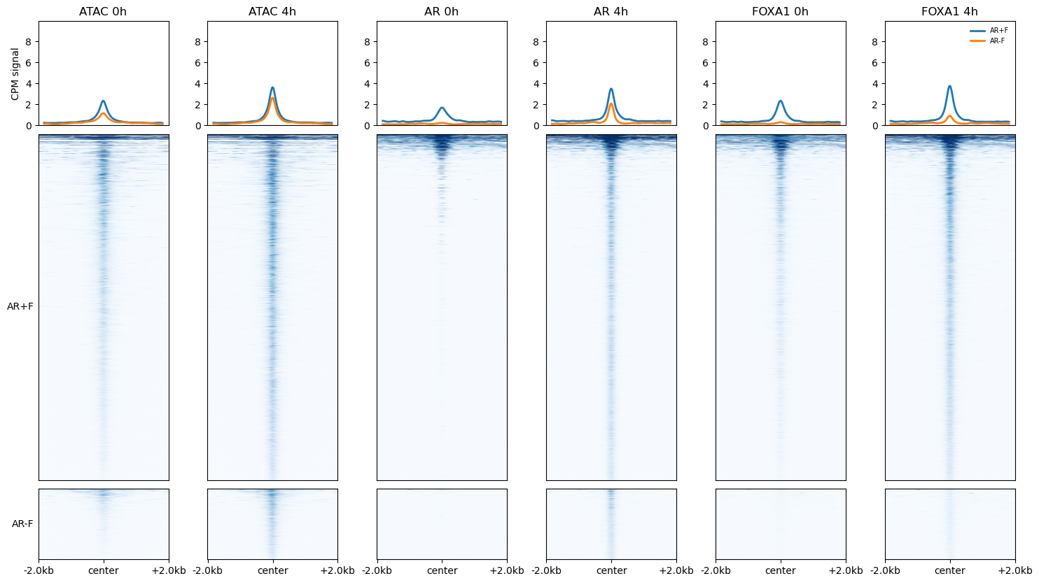
6. Signal heatmaps across conditions
Extract signal for AR+F and AR−F over all 8 bigwigs, average the two ATAC replicates per condition (the same averaging the browser does), and draw a grouped heatmap: ATAC 0h, ATAC 4h, AR 0h, AR 4h, FOXA1 0h, FOXA1 4h.
regions = ARpF + ARmF
groups  = {"AR+F": ARpF, "AR-F": ARmF}

bw_order = ["ATAC_0h_r1", "ATAC_0h_r2", "ATAC_4h_r1", "ATAC_4h_r2",
            "AR_0h", "AR_4h", "FOXA1_0h", "FOXA1_4h"]
bigwigs = [BW[k] for k in bw_order]

with timer("extract signal cube"):
    S = np.nan_to_num(regions.signal(bigwigs, n_bins=200, flank=2000, workers=4))
#S = tmm(np.nan_to_num(S))                       # per-track normalization

# group ATAC replicates by averaging their columns -> 6 conditions
S6 = np.stack([
    S[:, [0, 1], :].mean(1),   # ATAC 0h (rep1+rep2)
    S[:, [2, 3], :].mean(1),   # ATAC 4h (rep1+rep2)
    S[:, 4, :], S[:, 5, :],    # AR 0h, AR 4h
    S[:, 6, :], S[:, 7, :],    # FOXA1 0h, FOXA1 4h
], axis=1)
samples = ["ATAC 0h", "ATAC 4h", "AR 0h", "AR 4h", "FOXA1 0h", "FOXA1 4h"]
vmax = float(np.percentile(S6, 99))

with timer("draw heatmap"):
    fig = plot_heatmap(regions, S6, groups=groups, sets=["AR+F", "AR-F"],
                       samples=samples, vmax=vmax, ymax=vmax, height=2000)
▶ extract signal cube ...
[INFO] Extracting 8 bigwigs for 3027 loci into 200 bins (span=False, agg='mean', backend='pybigtools', exact=True, workers=4).


chunks: 100%|██████████| 4/4 [00:03<00:00,  1.26it/s]


✓ extract signal cube — 3.3s
▶ draw heatmap ...
✓ draw heatmap — 0.2s
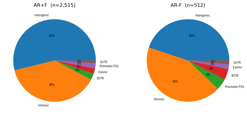
7. Genomic annotation of AR+F vs AR−F
with timer("load genes (GTF)"):
    genes = Genes.make(GTF)

with timer("annotate AR+F / AR-F"):
    annot_pf = genes.annotations(ARpF)
    annot_mf = genes.annotations(ARmF)

fig, axes = plt.subplots(1, 2, figsize=(9, 4))
for ax, df, title in [(axes[0], annot_pf, "AR+F"), (axes[1], annot_mf, "AR-F")]:
    vc = df["annotation"].value_counts()
    ax.pie(vc.values, labels=vc.index, autopct="%1.0f%%", textprops={"fontsize": 7})
    ax.set_title(f"{title}  (n={len(df):,})")
plt.tight_layout()
▶ load genes (GTF) ...
✓ load genes (GTF) — 8.1s
▶ annotate AR+F / AR-F ...
✓ annotate AR+F / AR-F — 0.7s
8. Motif enrichment — AR+F vs AR−F
Scan JASPAR motifs over AR+F, AR−F, and the accessible (ATAC) regions as the
background pool, then bootstrap the log-fold-change. Sorting by LFC
(= LFC_AR+F − LFC_AR−F) gives motifs preferential to each set. The scanners
read the windows from the FASTA through its index; to hold the genome in
memory instead, pass gb.read_fasta(GENOME_FA) in place of the path.
with timer("index genome FASTA"):
    genome = gb.Genome.from_fasta(GENOME_FA)     # builds hg38.fa.fai once; names and sizes

# background pool: every accessible region (the bootstrap draws 500 at a time)
pool = accessible

with timer("scan motifs (AR+F, AR-F, pool)"):
    mat_pf   = scan_motifs_matrix(ARpF, GENOME_FA, MOTIF_DB, r=250, workers=8)
    mat_mf   = scan_motifs_matrix(ARmF, GENOME_FA, MOTIF_DB, r=250, workers=8)
    mat_pool = scan_motifs_matrix(pool, GENOME_FA, MOTIF_DB, r=250, workers=8)

with timer("bootstrap enrichment"):
    enr = bootstrap_enrichment({"AR+F": mat_pf, "AR-F": mat_mf},
                               ref=mat_pool, boot=100, sample=500, seed=0)

show = ["Factor", "LFC", "LFC_AR+F", "LFC_AR-F"]
ranked = enr.sort_values("LFC", ascending=False)
print("Top motifs in AR+F (FOXA1-dependent):")
display(ranked.head(10)[show])
print("Top motifs in AR-F (FOXA1-independent):")
display(ranked.tail(10)[show].iloc[::-1])
▶ index genome FASTA ...
✓ index genome FASTA — 0.0s
▶ scan motifs (AR+F, AR-F, pool) ...


[motifs]: 100%|██████████| 33/33 [00:00<00:00, 47.91it/s]
[motifs]: 100%|██████████| 33/33 [00:00<00:00, 141.42it/s]


[motifs] 4 of 72470 windows run off a chromosome or are missing from the FASTA; their rows count 0.


[motifs]: 100%|██████████| 33/33 [00:18<00:00,  1.76it/s]


✓ scan motifs (AR+F, AR-F, pool) — 31.8s
▶ bootstrap enrichment ...


100%|██████████| 100/100 [00:00<00:00, 121.80it/s]
100%|██████████| 100/100 [00:00<00:00, 137.06it/s]
100%|██████████| 100/100 [00:00<00:00, 266.85it/s]


✓ bootstrap enrichment — 2.6s
Top motifs in AR+F (FOXA1-dependent):
| Factor | LFC | LFC_AR+F | LFC_AR-F | |
|---|---|---|---|---|
| 1439 | ZN671.H14CORE.0.P.C | 0.210842 | 0.201273 | -0.009569 |
| 1098 | TSH2.H14CORE.0.SG.A | 0.153191 | 0.149330 | -0.003861 |
| 240 | FOXA2.H14CORE.0.PSM.A | 0.126346 | 0.075877 | -0.050469 |
| 242 | FOXA3.H14CORE.0.PS.A | 0.108437 | 0.078202 | -0.030235 |
| 265 | FOXL2.H14CORE.0.PSM.A | 0.096419 | 0.069623 | -0.026797 |
| 266 | FOXM1.H14CORE.0.P.B | 0.091988 | 0.074143 | -0.017846 |
| 271 | FOXP1.H14CORE.0.PS.A | 0.091605 | 0.075136 | -0.016469 |
| 262 | FOXK1.H14CORE.0.PS.A | 0.089239 | 0.056245 | -0.032994 |
| 238 | FOXA1.H14CORE.0.P.B | 0.082882 | 0.052795 | -0.030086 |
| 1513 | ZN800.H14CORE.0.PSG.A | 0.075093 | 0.038774 | -0.036320 |
Top motifs in AR-F (FOXA1-independent):
| Factor | LFC | LFC_AR+F | LFC_AR-F | |
|---|---|---|---|---|
| 7 | ANDR.H14CORE.0.P.B | -0.152667 | 0.078639 | 0.231306 |
| 836 | PRGR.H14CORE.0.P.B | -0.091029 | 0.067898 | 0.158927 |
| 293 | GCR.H14CORE.0.PS.A | -0.085528 | 0.034008 | 0.119535 |
| 491 | KLF16.H14CORE.1.P.B | -0.079514 | -0.240093 | -0.160579 |
| 1559 | ZNF48.H14CORE.0.PSG.A | -0.071219 | -0.041029 | 0.030190 |
| 553 | MAZ.H14CORE.1.P.B | -0.070974 | -0.177320 | -0.106346 |
| 1122 | VEZF1.H14CORE.1.P.B | -0.063601 | -0.122012 | -0.058411 |
| 557 | MCR.H14CORE.0.S.B | -0.057377 | 0.027718 | 0.085095 |
| 1121 | VEZF1.H14CORE.0.P.C | -0.056297 | -0.148801 | -0.092504 |
| 506 | KMT2A.H14CORE.0.P.B | -0.053831 | -0.302884 | -0.249053 |
9. ChIP-Atlas (atlas) differential enrichment
Build a 1 kb bin × track index over the ChIP-Atlas hg38 collection, then use each region set as the other’s reference to find TF tracks differentially enriched between AR+F and AR−F.
Building the index over the full ChIP-Atlas is heavy (minutes, several GB RAM).
atlas.save("chipatlas_hg38_1kb.npz")/Atlas.load(...)reuse it across sessions.
with timer("build ChIP-Atlas index (1kb)"):
    atlas = Atlas.make(
        GIGGLE_DIR, chromsizes=CHROMSIZES,
        meta=GIGGLE_META,
        name_pattern=r"([^.]+)",                       # SRX23002840.20.bed.gz -> SRX23002840
        meta_columns=["id", "antigen", "class", "cell_line"],  # meta TSV is header-less
        meta_id_col="id",
    )

with timer("atlas search AR+F vs AR-F"):
    enr_pf = atlas.search(ARpF, ref=ARmF)    # enriched in AR+F over AR-F
    enr_mf = atlas.search(ARmF, ref=ARpF)    # enriched in AR-F over AR+F

cols = ["name", "antigen", "class", "cell_line", "overlaps", "log2_odds", "giggle_score"]
print("TF tracks enriched in AR+F (FOXA1-dependent):")
display(enr_pf.head(15)[cols])
print("TF tracks enriched in AR-F (FOXA1-independent):")
display(enr_mf.head(15)[cols])
▶ build ChIP-Atlas index (1kb) ...


[atlas index]: 100%|██████████| 33368/33368 [00:18<00:00, 1850.83it/s]


✓ build ChIP-Atlas index (1kb) — 42.5s
▶ atlas search AR+F vs AR-F ...
✓ atlas search AR+F vs AR-F — 5.0s
TF tracks enriched in AR+F (FOXA1-dependent):
| name | antigen | class | cell_line | overlaps | log2_odds | giggle_score | |
|---|---|---|---|---|---|---|---|
| 0 | SRX23002840 | FOXA1 | Prostate | LNCAP | 1329 | 7.519583 | 964.923631 |
| 1 | SRX23002841 | FOXA1 | Prostate | LNCAP | 1089 | 7.056433 | 700.212091 |
| 2 | SRX18285237 | FOXA1 | Prostate | LNCAP | 1847 | 4.287255 | 618.551089 |
| 3 | SRX14353424 | FOXA1 | Prostate | LNCAP | 1990 | 4.058525 | 604.652460 |
| 4 | SRX18285235 | FOXA1 | Prostate | LNCAP | 1722 | 4.333244 | 580.711304 |
| 5 | SRX062360 | FOXA1 | Prostate | LNCAP | 1564 | 4.546911 | 564.964852 |
| 6 | SRX14353423 | FOXA1 | Prostate | LNCAP | 1756 | 4.155838 | 548.736062 |
| 7 | SRX5577144 | Epitope tags | Prostate | LNCAP | 1779 | 4.090175 | 540.034633 |
| 8 | SRX1885188 | FOXA1 | Prostate | LNCAP | 2044 | 3.775184 | 533.691700 |
| 9 | SRX18285236 | FOXA1 | Prostate | LNCAP | 1470 | 4.498439 | 515.002750 |
| 10 | SRX1885186 | FOXA1 | Prostate | LNCAP | 1936 | 3.774294 | 503.551086 |
| 11 | SRX1885187 | FOXA1 | Prostate | LNCAP | 1878 | 3.818223 | 499.236335 |
| 12 | SRX1885185 | FOXA1 | Prostate | LNCAP | 1972 | 3.724534 | 499.063986 |
| 13 | SRX1212235 | FOXA1 | Prostate | LNCAP | 1936 | 3.749926 | 496.615360 |
| 14 | SRX6878606 | FOXA1 | Prostate | LNCAP | 1877 | 3.763680 | 484.060928 |
TF tracks enriched in AR-F (FOXA1-independent):
| name | antigen | class | cell_line | overlaps | log2_odds | giggle_score | |
|---|---|---|---|---|---|---|---|
| 0 | SRX3070471 | NR3C1 | Breast | MCF 10A | 151 | 1.985641 | 57.274594 |
| 1 | SRX3070475 | NR3C1 | Breast | MCF 10A | 120 | 2.021899 | 49.016228 |
| 2 | SRX21439743 | ESR1 | Prostate | LNCAP | 452 | 1.518987 | 46.612336 |
| 3 | SRX3070473 | NR3C1 | Breast | MCF 10A | 120 | 1.969408 | 45.866518 |
| 4 | SRX306516 | AR | Prostate | DU 145 | 161 | 1.690385 | 39.808143 |
| 5 | SRX19970679 | AR | Prostate | PC-346C | 167 | 1.537133 | 31.894465 |
| 6 | SRX8520802 | NR3C1 | Breast | HCC1187 | 173 | 1.506006 | 31.057426 |
| 7 | SRX21439744 | ESR1 | Prostate | LNCAP | 336 | 1.292770 | 30.240255 |
| 8 | SRX3070469 | NR3C1 | Breast | MCF 10A | 53 | 2.255766 | 30.173945 |
| 9 | SRX21439742 | ESR1 | Prostate | LNCAP | 295 | 1.284194 | 28.358706 |
| 10 | SRX083218 | AR | Prostate | LNCAP | 236 | 1.337458 | 28.128496 |
| 11 | SRX1067071 | AR | Prostate | LHSAR | 319 | 1.253582 | 27.290928 |
| 12 | SRX1067070 | AR | Prostate | LHSAR | 340 | 1.245091 | 27.235381 |
| 13 | SRX083219 | AR | Prostate | LNCAP | 233 | 1.311355 | 26.426950 |
| 14 | SRX3630817 | NR3C1 | Uterus | Ishikawa | 53 | 2.092061 | 25.168441 |
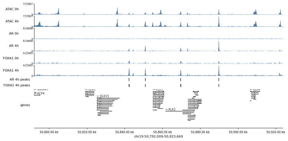
10. Browser view — chr19:50,792,009-50,923,669
All six conditions as signal tracks (ATAC replicates passed as a list of bigwigs are averaged into one track), their peak calls, and gene models. The region string is 0-based, half-open like every table.
region = "chr19:50,792,009-50,923,669"
tracks = {
    "ATAC 0h":   [BW["ATAC_0h_r1"], BW["ATAC_0h_r2"]],   # list -> averaged
    "ATAC 4h":   [BW["ATAC_4h_r1"], BW["ATAC_4h_r2"]],
    "AR 0h":     BW["AR_0h"],
    "AR 4h":     BW["AR_4h"],
    "FOXA1 0h":  BW["FOXA1_0h"],
    "FOXA1 4h":  BW["FOXA1_4h"],
    "AR 4h peaks":    PEAK["AR_4h"],
    "FOXA1 4h peaks": PEAK["FOXA1_4h"],
    "genes":     genes,
}
# share the y-axis within each assay so the 0h -> 4h gain is honest
with timer("browser render"):
    fig, axes = browser(region, tracks, bw_n_bins=2000, figsize=(11, None),
                        bw_share=[["ATAC 0h", "ATAC 4h"],
                                  ["AR 0h", "AR 4h"],
                                  ["FOXA1 0h", "FOXA1 4h"]])
▶ browser render ...
✓ browser render — 1.0s