Browser

Three ways to look at a region. gb.browser draws a vector figure with matplotlib; gb.igv_html writes one HTML file that opens igv.js on your data; gb.View writes one HTML file with genomeblocks’ own interactive viewer, which knows the tables. All three take the same tables and the same region strings.

Table of contents

1. Which viewer
   1. Region strings
2. gb.browser — a matplotlib region view
   1. bigWig tracks
   2. BAM tracks and the reference sequence
   3. Genes
   4. Layout and styling
3. gb.igv_html — one HTML file that opens IGV
4. gb.View — the one-file interactive view
5. Real example
6. Tips

---

Which viewer

	gb.browser	gb.igv_html	gb.View
Output	matplotlib Figure (SVG / PDF / PNG)	one .html file, igv.js	one .html file, our canvas viewer
Needs	matplotlib	a web browser (igv.js from a CDN, or embedded)	a web browser, nothing else
Best for	figures for a paper	sharing with people who use IGV; BAM / VCF review	browsing hubs: search a gene, see its anchor CREs, partners and O/E per sample
Tracks	bigWig, BAM, intervals, Pairs, Genes	intervals, Genes, bigWig, Architecture loops	profiles, bigWig, intervals, points, CREs, loops, Genes
Data scope	the region	genome-wide intervals and genes; signal and loops around the listed regions	genome-wide, with fine signal bins around the listed regions

Region strings

Every viewer parses regions the same way (genomeblocks.locus.parse_region):

"chr6:122,600,000-122,800,000"       # thousands separators
"chr8:127.7-128.1 Mb"                # kb / Mb units on either number
"chr2:5kb-12kb"
("chr6", 122_600_000, 122_800_000)   # a tuple
gb.Loci.make("cre.bed")[0]           # a Locus / LocusView

igv_html and View also accept two regions in one string ("chr8:127.7-128.0 Mb chr1:1-2 Mb") for a split view.

---

gb.browser — a matplotlib region view

One call, one sub-axes per track plus a coordinate ruler. The track kind is detected from the value:

import genomeblocks as gb

cre   = gb.Loci.make("cre.bed")
genes = gb.Genes.make("genes.gtf")
pairs = gb.Pairs.make("loops.bedpe")

fig, axes = gb.browser(
    "chr1:0-12 kb",
    tracks={
        "ATAC":           "atac.bw",                      # a bigWig path
        "ATAC + H3K27ac": ["atac.bw", "h3k27ac.bw"],      # a list: averaged into one track
        "CREs":           cre,                            # a Loci
        "frame":          cre.to_pandas(),                # any frame as_loci reads
        "peaks":          "cre.bed",                      # a BED / narrowPeak path
        "loops":          pairs,                          # a Pairs ...
        "loops file":     "loops.bedpe",                  # ... or a BEDPE path
        "regions":        ["chr1:500-700", "chr1:3000-3500"],   # a list of regions
        "genes":          genes,                          # gene models
    },
    bw_share=[["ATAC", "ATAC + H3K27ac"]],
    colors={"loops": "#DA0000", "ATAC": "#4c78a8"},
    genes_max_transcripts=1,
)
fig.savefig("region.svg")
list(axes)
# -> ['ATAC', 'ATAC + H3K27ac', 'CREs', 'frame', 'peaks', 'loops', 'loops file', 'regions', 'genes', '_axis']

Track value	Detected as	Rendered as
*.bw, *.bigwig path, or an open pyBigWig / pybigtools handle	bw	binned coverage: fill_between + a step outline
a list of bigWig paths / handles	bw	one averaged track (replicate grouping)
*.bam path	bam	per-base depth with IGV-style mismatch colouring (needs reference=)
*.bedpe path or a Pairs	bedpe	half-sine arcs between anchor midpoints; line width follows score
a Genes	genes	stacked gene models: body line, exon boxes, taller CDS boxes, name and strand arrow
anything else as_loci reads: Loci, BED / narrowPeak path, pandas / polars / arrow frame, a region string, a list of regions	bed	one row of rectangles

Only the region is read: bigWigs give bw_n_bins binned values, intervals and genes are looked up by overlap.

Every track is its own axis on one x range. browser() picks the drawer from the value — a bigWig path becomes binned means of the region only (one native call through the bigwig backend), a list of bigWigs is averaged per bin, anything as_loci reads becomes a row of rectangles, a Pairs or BEDPE path becomes arcs between anchor midpoints, a Genes becomes stacked models from its three tables — and stacks them over a shared ruler, so you mix sources without converting anything first.

bigWig tracks

fig, axes = gb.browser("chr1:0-12 kb", {"AR 0h": "ar_0h.bw", "AR 4h": "ar_4h.bw", "ATAC": "atac.bw"},
                       bw_n_bins=1000,                   # bins per track across the region (default 1000)
                       bw_ymax={"ATAC": 150.0},          # a scalar for every bigWig track, or per track
                       bw_share=[["AR 0h", "AR 4h"]],    # groups that share one y-scale (the group's region max)
                       backend="python")                 # bigWig engine: 'pybigtools' (default), 'pybigwig', 'python'
axes["AR 0h"].get_ylim() == axes["AR 4h"].get_ylim()
# -> True

An explicit bw_ymax wins over bw_share; otherwise each track is scaled to its own region maximum. Open handles are read with their own library, so backend= applies to paths only (see Signal).

BAM tracks and the reference sequence

A BAM track needs a coordinate-sorted .bam with its .bai alongside, pysam (pip install genomeblocks[bam]), and an indexed FASTA passed as reference= (.fa + .fai):

fig, axes = gb.browser(
    "chr7:5,527,000-5,530,000",
    tracks={"WGS": "sample.bam", "CREs": cre},
    reference="hg38.fa",
    bam_min_baseq=15,          # IGV default
    bam_allele_freq=0.2,       # colour a position once ≥ 20% of its reads mismatch the reference
    bam_ymax=None,             # scalar or per track; bam_share=[[...]] groups scales as for bigWigs
    show_sequence=True,        # a reference-sequence track above the ruler (letters ≤ 200 bp, a strip ≤ 5 kb)
)
list(axes)
# -> ['WGS', 'CREs', '_sequence', '_axis']

Total depth is a gray step; positions above bam_allele_freq get nucleotide-coloured bars for the mismatching reads. A BAM track without reference= raises before anything is drawn. gb.coverage(bam, region) gives the same per-base depth as an array.

Genes

genes_max_transcripts=1 collapses each gene to one isoform — the canonical one when Genes.select_isoforms has run, else the longest; None (default) stacks every isoform. Transcripts are packed greedily into rows; exons are thin boxes, CDS taller boxes, and each gene gets a label with a strand arrow.

Layout and styling

arg	meaning
figsize=(w, h)	h=None (default) derives the height from the track heights
track_heights={name: inches}	defaults: bigWig 0.5, BAM 0.6, intervals 0.2, loops 1.5, genes 1.5, sequence 0.2 ('_sequence')
colors={name: "#hex"}	per-track colour
label_fontsize, hspace, dpi	cosmetics

Returns (fig, axes_by_name). axes_by_name['_axis'] is the ruler and '_sequence' the reference track, so you can overlay annotations on any track before saving. The output is SVG-clean: coverage is fill_between, intervals are PatchCollections of rectangles, arcs are LineCollections — no rasterized patches, small files that open in Inkscape or Illustrator.

A region whose end is not after its start raises:

gb.browser("chr1:100-50", {"CREs": cre})
# -> ValueError: Invalid region: end (50) must be > start (100)

---

gb.igv_html — one HTML file that opens IGV

A = (gb.Architecture.make(cre, "loops.bedpe", r=100)
       .add_mcool("hic.mcool", resolution=5000).normalize())

sizes = gb.igv_html(
    "share.html",
    regions=["chr1:0-12 kb",                       # one-click buttons; strings, tuples or Locus
             "chr1:0-5 kb chr2:1-6 kb",            # two loci in one string: a split view (a trans loop)
             ("chr1", 0, 5000)],
    loci={"CREs": cre, "frame": cre.to_pandas()},  # {track: anything as_loci reads}, embedded genome-wide
    genes=genes,                                   # one BED12 model per gene, genome-wide
    signal={"ATAC": "atac.bw"},                    # {track: bigWig path or open handle}, around the regions only
    architecture=A, score="n",                     # loops touching the regions, arc height = ep[score]
    notes={"chr1:0-12 kb": "GENE_A and GENE_B"},   # one line under a button
    title="demo",
)
sizes
# -> {'ATAC': 2005, 'CREs': 197, 'frame': 197, 'loops (n)': 149, 'genes': 185, 'total': 7312}

Every track is embedded in the page as a gzipped data URI and igv.js draws it. The reader needs nothing but a web browser. Size is the only limit: loci and genes are embedded genome-wide, signal and architecture loops only for the listed regions ± flank (default 250 kb), at bin_size bp (default 50). The returned dict is the size of each track in bytes.

Regions are parsed with units and thousands separators and written 1-based for igv.js (chr1:0-5 kb becomes chr1:1-5000). The first region is the opening view; users can still type any locus or gene name.

arg	meaning
chrom_sizes	{chrom: length}; default: the sizes in the bigWig headers, and for a chromosome no bigWig names, the extent of the embedded loci / architecture and the regions plus flank
genome_id	e.g. 'hg38': use igv.js’s hosted genome (sequence, ideogram, gene search) instead of embedded sizes; needs internet
igv_js	'cdn' (default: jsDelivr, the page stays small), a path to a local igv.min.js to embed (~1.5 MB, works fully offline), or any URL
standalone	False writes the page content without <html> / <head> for hosts that add their own
backend	bigWig engine for signal
subtitle	one line under the title

igv_html is the export for BAM / VCF review or very large remote files, and for readers who already know IGV. For the tables themselves — hubs, anchors, partners, O/E per sample — gb.View can do more because it knows what a CRE and an edge are.

---

gb.View — the one-file interactive view

View writes one HTML file: the same columns genomeblocks keeps in memory (gzipped typed arrays) plus a small canvas viewer. No install, no server, works offline. Because the viewer knows the tables, a gene search lights up its anchor CREs (TSS ± anchor_r), draws the anchor’s contact profile per sample, lists partners with their O/E, and opens a trans partner side by side.

Build it like a figure: one track per method call, drawn in call order.

A.annotate(genes).strength()

v = gb.View(A, genes=genes,
            samples={"LNCaP": "#46a8e4", "VCaP": "#ffa600"},    # sample -> colour (a list gets automatic colours)
            title="MYC hubs", subtitle="HiChIP O/E, two lines",
            anchor_r=5000, gene_half=500_000)

v.anchor_profile("contacts of the anchor (O/E)")                # per-sample edge weight from the anchor to every partner
v.cre_values("node strength", {"LNCaP": A.vp.strength,          # per-CRE numbers, aligned to the CRE rows
                               "VCaP": A.vp.strength_vcap})
v.signal("ATAC", {"LNCaP": "atac_lncap.bw", "VCaP": "atac_vcap.bw"},
         bin_size=50, flank=250_000, genome_bin=20_000)         # fine bins around the regions, coarse bins genome-wide
v.intervals("super-enhancers", {"LNCaP": se_lncap, "VCaP": se_vcap})   # a Loci / frame / path per sample ...
v.intervals("promoters", A.vp.annot == "Promoter-TSS", color="#2a9d8f")  # ... or a boolean mask over the CRE rows
v.points("copy number", {"LNCaP": "lncap.cnr"}, value="log2", ylim=(-2, 2))   # chromosome/start/end/value tables
v.cres()                                                        # the CRE rows; promoters darker, anchor and partners highlighted
v.loops({"LNCaP": "n", "VCaP": "n_vcap"})                       # edges as arcs; an edge column per sample
v.genes()

v.region("MYC", gene="MYC", note="the anchor")                  # a one-click button; gene= anchors that gene
v.region("E-MYC and its trans partner", "chr8:127.7-128.0 Mb chr1:1-2 Mb")   # two loci: split view
v.mark("E-MYC", "chr8", 127_734_800)                            # a labelled position
v.hubs(A.vp.strength, n=12, label="strength")                   # the 'Top hubs' list

parts = v.save("myc.html")                                      # bytes per part
v                                                               # in a notebook: the page in an iframe

Method	Track
anchor_profile(name, smooth=1.5)	sum of edge weight from the selected gene / CRE to every partner, per sample
cre_values(name, values, smooth=1.0)	one number per CRE row, drawn as a profile; {sample: array} overlays
signal(name, bigwigs, bin_size=50, flank=250_000, genome_bin=20_000)	bigWig (path or handle, or {sample: path}): fine bins around the listed regions, coarse max bins genome-wide
intervals(name, sets, color=None)	interval rows: a Loci or anything as_loci reads, a boolean mask over the CRE rows, or {sample or label: ...}
points(name, tables, chrom="chromosome", start="start", end="end", value="log2", segments=None, ylim=None)	values along the genome (CNVkit .cnr columns by default; a path is read as TSV), optional labelled segments
cres(name="CREs")	the CRE rows
loops(score="n", name="loops")	edges as arcs, trans edges as labelled stubs; score is an edge column or {sample: column} (needs an Architecture)
genes(name="genes")	one transcript per gene: the canonical isoform when selected, else the longest

Navigation: region(label, locus=None, gene=None, note="", anchor=None) adds a button (with gene= and no locus, the view is TSS ± gene_half); mark(label, chrom, pos) adds a labelled position; hubs(values, n=12, label=None) fills the “Top hubs” list with the n CRE rows with the largest values (when vp.strength exists and hubs is not called, strength is used).

View(cre=...) works without an Architecture for signal, intervals, points and genes; loops raises without one, and anchor_profile has no edges to sum. A View with no tracks added gets a default figure on save: anchor profile, node strength, CREs, loops, genes. genomeblocks.view.view_html(path, architecture=, genes=, signal=, regions=) is that default figure in one call.

parts = v.save("myc.html")
# -> {'CREs': 224, 'edges': 180, 'genes': 366, 'track: node strength': 120, 'track: ATAC': 5248, ..., 'viewer (js + css)': 43118, 'total': 54666}

Chromosome lengths come from the Loci’s Genome when it has sizes (Genome.from_sizes, Loci.tile_genome), else from the furthest interval plus 250 kb; pass chrom_sizes= (a path or a dict) for the real ones.

---

Real example

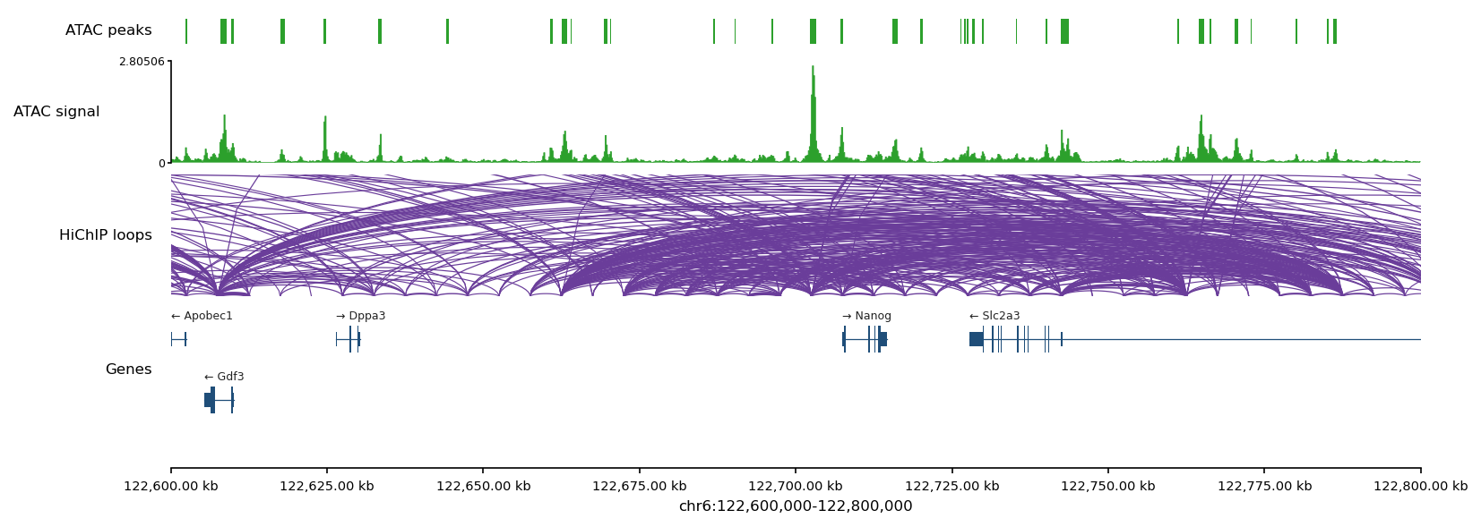
The Nanog locus (mm10) rendered with gb.browser: HiChIP loops, ATAC signal, ATAC peaks, and GENCODE protein-coding genes:

A complete, runnable real-data example (AR & FOXA1 in LNCaP) lives in examples/ar_foxa1_lncap/ and is walked through step by step in the AR & FOXA1 example.

---

Tips

• For wide regions, drop bw_n_bins to 120–240 to keep the SVG small without losing the profile shape.
• gb.browser reads only the region, so it is cheap on genome-wide bigWigs; igv_html and View embed data, so list only the regions you need and keep flank modest.
• Use the same samples dict across several Views so colours stay consistent between figures.